e-Discovery Team

This is the fourth of seven informal video talks on document review and predictive coding. The first video explained why this is important to the future of the Law. The second talked about ESI Communications. The third about Multimodal Search Review. This video talks about the third step of the e-Discovery Team’s eight-step work flow, shown above, Random Baseline Sample.

Although this text intro is overly long, the video itself is short, under eight minutes, as there is really not that much to this step. You simply take a random sample at or near the beginning of the project. Again, this step can be used in any document review project, not just ones with predictive coding. You do this to get some sense of the prevalence of  relevant documents in the data collection. That just means the sample will give you an idea as to the total number of relevant documents. You do not take the sample to set up a secret control set, a practice that has been thoroughly discredited by our Team and others. See Predictive Coding 3.0.

If you understand sampling statistics you know that sampling like this produces a range, not an exact number. If your sample size is small, then the range will be very high. If you want to reduce your range in half, which is a function in statistics known as a confidence interval, you have to quadruple your sample size. This is a general rule of thumb that I explained in tedious mathematical detail several years ago in Random Sample Calculations And My Prediction That 300,000 Lawyers Will Be Using Random Sampling By 2022. Our Team likes to use a fairly large sample size of about 1,533 documents that creates a confidence interval of plus or minus 2.5%, subject to a confidence level of 95% (meaning the true value will lie within that range 95 times out of 100). More information on sample size is summarized in the graph below. Id.

The picture below this paragraph illustrates a data cloud where the yellow dots are the sampled documents from the grey dot total, and the hard to see red dots are the relevant documents found in that sample. Although this illustration is from a real project we had, it shows a dataset that is unusual in legal search because the prevalence here was high, between 22.5% and 27.5%. In most data collections searched in the law today, where the custodian data has not been filtered by keywords, the prevalence is far less than that, typically less than 5%, maybe even less that 0.5%. The low prevalence increases the range size, the uncertainties, and requires a binomial calculation adjustment to determine the statistically valid confidence interval, and thus the true document range.

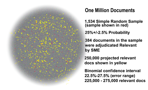
For example, in a typical legal project with a few percent prevalence range, it would be common to see a range between 20,000 and 60,000 relevant documents in a 1,000,000 collection. Still, even with this very large range, we find it useful to at least have some idea of the number of documents they are looking for. That is what the Baseline Step can provide to you, nothing more nor less.

If you are unsure of how to do sampling for prevalence estimates, your vendor can probably help. Just do not let them tell you that it is one exact number. That is simply a point projection near the middle of a range. The one number point projection is just the top of the typical probability bell curve shown above, which illustrates a 95% confidence level distribution. The top is just one possibility, albeit slightly more likely than either end points. The true value could be anywhere in the blue range.

To repeat, the Step Three prevalence baseline number is always a range, never just one number. Going back to the relatively high prevalence example, the below bell cure shows a point projection of 25% prevalence, with a range of 22.2% and 27.5%, creating a range of relevant documents of from between 225,000 and 275,000. This is shown below.

The important point that many vendors and other “experts” often forget to mention, is that you can never know exactly where within that range the true value may lie. Plus, there is always a small possibility, 5% when using a sample size based on a 95% confidence level, that the true value may fall outside of that range. It may, for example, only have 200,000 relevant documents. This means that even with a high prevalence project with datasets that approach the Normal Distribution of 50% (here meaning half of the documents are relevant), you can never know that there are exactly 250,000 documents, just because it is the mid-point or point projection. You can only know that there are between 225,000 and 275,000 relevant documents, and even that range may be wrong 5% of the time. Those uncertainties are inherent limitations to random sampling.

Shame on the vendors who still perpetuate that myth of certainty. Lawyers can handle the truth. We are used to dealing with uncertainties. All trial lawyers talk in terms of probable results at trial, and risks of loss, and often calculate a case’s settlement value based on such risk estimates. Do not insult our intelligence by a simplification of statistics that is plain wrong. Reliance on such erroneous point projections alone can lead to incorrect estimates as to the level of recall that we have attained in a project. We do not need to know the math, but we do need to know the truth.

The short video that follows will briefly explain the Random Baseline step, but does not go into the technical details of the math or statistics, such as the use of the binomial calculator for low prevalence. I have previously written extensively on this subject. See for instance:

• In Legal Search Exact Recall Can Never Be Known
• Random Sample Calculations And My Prediction That 300,000 Lawyers Will Be Using Random Sampling By 2022
• Borg Challenge: Part Two where I begin the search with a random sample (text and video)

If you prefer to learn stuff like this by watching cute animated robots, then you might like: Robots From The Not-Too-Distant Future Explain How They Use Random Sampling For Artificial Intelligence Based Evidence Search. But be careful, their view is version 1.0 as to control sets.

Thanks again to William Webber and other scientists in this field who helped me out over the years to understand the Bayesian nature of statistics (and reality).

For details on all eight steps, including this third step, see Predictive Coding 3.0. More information on document review and predictive coding can be found in the fifty-six articles published here.

______

___

This entry was posted on Friday, March 11th, 2016 at 8:55 am and is filed under Lawyers Duties, Review, Search, Technology, VENDORS. You can follow any responses to this entry through the RSS 2.0 feed. You can leave a response, or trackback from your own site.