TAR Course: 13th Class

Thirteenth Class: Step Three – Random Prevalence

There has been no change in this step from Version 3.0 to Version 4.0. The third step, which is not necessarily chronological, is essentially a computer function with statistical analysis. Here you create a random sample and analyze the results of expert review of the sample. Some review is thus involved in this step and you have to be very careful that it is correctly done. This sample is taken for statistical purposes to establish a baseline for quality control in step seven. Typically prevalence calculations are made at this point. Some software also uses this random sampling selection to create a control set. As explained at length in Predictive Coding 3.0, we do not use a control set because it is so unreliable. It is a complete waste of time and money and does not produce reliable recall estimates. Instead, we take a random sample near the beginning of a project solely to get an idea on Prevalence, meaning the approximate number of relevant documents in the collection.

Unless we are in a very rushed situation, such as in the TREC projects, where we would do a complete review in a day or two, or sometimes just a few hours, we like to take the time for the sample and prevalence estimate.

It is all about getting a statistical idea as to the range of relevant documents that likely exist in the data collected. This is very helpful for a number of reasons, including proportionality analysis (importance of the ESI to the litigation and cost estimates) and knowing when to stop your search, which is part of step seven. Knowing the number of relevant documents in your dataset can be very helpful, even if that number is a range, not exact. For example, you can know from a random sample that there are between four thousand and six thousand relevant documents. You cannot know there are exactly five thousand relevant documents. See: In Legal Search Exact Recall Can Never Be Known. Still, knowledge of the range of relevant documents (red in the diagram below) is helpful, albeit not critical to a successful search.

Prevalence_binomial_gaussian

In step three an SME is only needed to verify the classifications of any grey area documents found in the random sample. The random sample review should be done by one reviewer, typically your best contract reviewer. They should be instructed to code as Uncertain any documents that are not obviously relevant or irrelevant based on their instructions and step one. All relevance codings should be double checked, as well as Uncertain documents. The senior SME is only consulted on an as-needed basis.

Document review in step three is limited to the sample documents. Aside from that, this step is a computer function and mathematical analysis. Pretty simple after you do it a few times. If you do not know anything about statistics, and your vendor is also clueless on this (rare), then you might need a consulting statistician. Most of the time this is not necessary and any competent Version 4.0 vendor expert should be able to help you through it.

It is not important to understand all of the math, just that random sampling produces a range, not an exact number. If your sample size is small, then the range will be very high. If you want to reduce your range in half, which is a function in statistics known as a confidence interval, you have to quadruple your sample size. This is a general rule of thumb that I explained in tedious mathematical detail several years ago in Random Sample Calculations And My Prediction That 300,000 Lawyers Will Be Using Random Sampling By 2022. Our Team likes to use a fairly large sample size of about 1,533 documents that creates a confidence interval of plus or minus 2.5%, subject to a confidence level of 95% (meaning the true value will lie within that range 95 times out of 100). More information on sample size is summarized in the graph below. Id.

Here is a recent example of how this worked in an actual employment claim matter. We took a simple random sample of 1,535 documents from a total collection of 729,569 documents. We then reviewed these very carefully. There were no serious undetermined documents and so the SME delegates, a paralegal and associate working on the case, were able to check the review. There was no need to bring in the head SME partner to look at any of these. After carefully checking we determined that the sample set contained 45 relevant and 1,490 not relevant.

With the 1,535 sample, which is based on a 95% Confidence Level and Confidence Interval of 2.5%, the spot projection (most likely) is a Prevalence of 3.02%, with a binomial confidence interval range of from between 2.21% to 4.02%. This means that 95 times out of a hundred (Confidence Level) there will be between 16,258 to 29,574 relevant Documents in this collection, with the highest probability of 22,217 Relevant documents. This sampling review and Prevalence range calculation helps guide us on the document review. Review of the random sample helps give us an overview of the collection. The prevalence range knowledge helps us to evaluate the scope and burden, and later in the stop decision.

The picture below this paragraph illustrates a data cloud of another project where the yellow dots are the sampled documents from the grey dot total, and the hard to see red dots are the relevant documents found in that sample. Although this illustration is from another real project we had, it shows a data-set that is unusual in legal search because the prevalence here was high, between 22.5% and 27.5%.

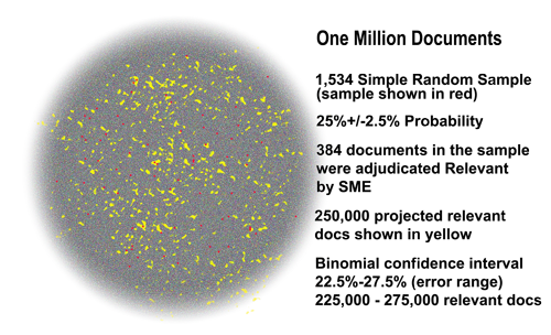
In most data collections searched in the law today, where the custodian data has not been filtered by keywords, the prevalence is far less than that, typically less than 5%, maybe even less that 0.5%. As noted in the prior example, the prevalence range was from between 2.21% to 4.02%, with the most likely prevalence of 3.02%.

The low prevalence increases the range size, the uncertainties, and requires a binomial calculation adjustment to determine the statistically valid confidence interval, and thus the true document range.

For another example, in a typical legal project with a few percent prevalence range, it would be common to see a range between 20,000 and 60,000 relevant documents in a 1,000,000 collection. Still, even with this very large range, we find it useful to at least have some idea of the number of relevant documents that we are looking for. That is what the Baseline step can provide to you, nothing more nor less.

As mentioned, your vendor can probably help you with these statistical estimates. Just do not let them tell you that it is one exact number. It is always a range. The one number approach is just a shorthand for the range. It is simply a point projection near the middle of the range. The one number point projection is the top of the typical probability bell curve range shown right, which illustrates a 95% confidence level distribution. The top is just one possibility, albeit slightly more likely than either end points. The true value could be anywhere in the blue range.

To repeat, the step three prevalence baseline number is always a range, never just one number. Going back to the relatively high prevalence example, the below bell cure shows a point projection of 25% prevalence, with a range of 22.2% and 27.5%, creating a range of relevant documents of from between 225,000 and 275,000. This is shown below.

The important point that many vendors and other “experts” often forget to mention, is that you can never know exactly where within that range the true value may lie. Plus, there is always a small possibility, 5% when using a sample size based on a 95% confidence level, that the true value may fall outside of that range. It may, for example, only have 200,000 relevant documents. This means that even with a high prevalence project with datasets that approach the Normal Distribution of 50% (here meaning half of the documents are relevant), you can never know that there are exactly 250,000 documents, just because it is the mid-point or point projection. You can only know that there are between 225,000 and 275,000 relevant documents, and even that range may be wrong 5% of the time. Those uncertainties are inherent limitations to random sampling.

Shame on the vendors who still perpetuate that myth of certainty. Lawyers can handle the truth. We are used to dealing with uncertainties. All trial lawyers talk in terms of probable results at trial, and risks of loss, and often calculate a case’s settlement value based on such risk estimates. Do not insult our intelligence by a simplification of statistics that is plain wrong. Reliance on such erroneous point projections alone can lead to incorrect estimates as to the level of recall that we have attained in a project. We do not need to know the math, but we do need to know the truth.

The short video that follows will briefly explain the Random Baseline step, but does not go into the technical details of the math or statistics, such as the use of the binomial calculator for low prevalence. I have previously written extensively on this subject. See for instance:

If you prefer to learn stuff like this by watching cute animated robots, then you might like: Robots From The Not-Too-Distant Future Explain How They Use Random Sampling For Artificial Intelligence Based Evidence Search. But be careful, their view is version 1.0 as to control sets.

Thanks again to William Webber and other scientists in this field who helped me out over the years to understand the Bayesian nature of statistics (and reality).

_______

_____

We close this class with an example to illustrate how this prevalence step works. Below is a screen shot of a project Ralph was working on in 2017 using KrolLDiscovery software. In the video that follows Ralph explains the prevalence calculation made in that case and how it helped guide his efforts. You will see another video discussing this case at the end of the next class.

By the way, Ralph misspoke in the video at point 8:39 when he said 95% confidence interval, he meant to say 95% confidence level. The random sample of 1,535 documents created a probability of 95% +/- 2.5%, meaning a 95% confidence level subject to an error range or interval of plus or minus 2.5%.

___

Go on to the Fourteenth Class.

Or pause to do this suggested “homework” assignment for further study and analysis.

SUPPLEMENTAL READING: It is important to read the cited article, In Legal Search Exact Recall Can Never Be Known. Also look at the few links in that article. Sometimes you need to reread these math-filled articles several times to pick it up. So unless you are a math wiz, take your time with this and do not get discouraged. It will eventually sink in. Also, at least skim the more math based article cited in this class, Random Sample Calculations And My Prediction That 300,000 Lawyers Will Be Using Random Sampling By 2022. I suggest you actually try out the math yourself and see how it works. Create your own examples to try it out. It is all multiplication and division and only requires an understanding of proportions. It is far easier than you might think. The hardest part is learning to think in terms of probability not certainty, but that is how lawyers have always evaluated case outcomes, so it is not entirely new for most attorneys.

If you talk about recall calculations based on sampling than you must also talk about range of recall estimates due to inherent sampling error. To simply say you attained an exact spot projection is inaccurate. This is what separates the amateurs from the pros in predictive coding. All students of the TAR Course need to understand how sampling necessarily results in a range of probabilities, never an exact number. That is due to the Confidence Interval. Hopefully you can also make these calculations for yourself, but if not, at least understand probabilities from sampling and the margin of error. To deepen your understanding we recommend that you find and read basic articles on statistics and random sampling. Be sure that you understand the Confidence Level and Confidence Interval. Try to find discussions on the Binomial Confidence Interval, and the difference with Gaussian Confidence Interval, and why Binomial is preferred in low prevalence samples.

EXERCISES: On the right column of this e-Discovery Team blog you will find a box that says MATH TOOLS FOR QC (shown right). It has links to the two most important math tools needed for this and other classes in the TAR Course, a random sample size calculator and a binomial confidence interval calculator. Click on the links, study the resources and further links on those two math tool pages. Then try out these tools by entering many different values and observing the impact. Try using these tools in your next document review project to calculate prevalence range. It does not have to be a predictive coding project. This step can be useful in any type of document review.

By the way, no one uses a 99% Confidence Level. Always use the 95% Confidence Level. That is what is used in scientific experiments and medical research. To increase certainty and tighten the size of the probability range, it is better to lower the Confidence Interval, not increase the Confidence Level. I typically use a 2.5% Confidence Interval with a 95% Confidence Level. That is written out like this: 95% +/- 2.5%. In a smaller case I may increase the percentage of the Confidence Interval to 3.0%, maybe even as high as 5%. If you go higher than that, the error range is so high that the information has little value. Besides, it does not take a large sample to meet the 95% +/- 5% specification. How many does it take? What is the sample size needed for various intervals in a document collection of 100,000? Let’s get specific: how many documents do you need in a sample to meet my favorite specification of a 2.5% Confidence Interval, and 95% Confidence Level, in a collection of one million documents? Same question for ten thousand documents? For ten million? For a trillion?! Note the small variance of the sample size required. For me that is the amazing power of random sampling.

Students are invited to leave a public comment below. Insights that might help other students are especially welcome. Let’s collaborate!